Introduction to Statistics
Introduction
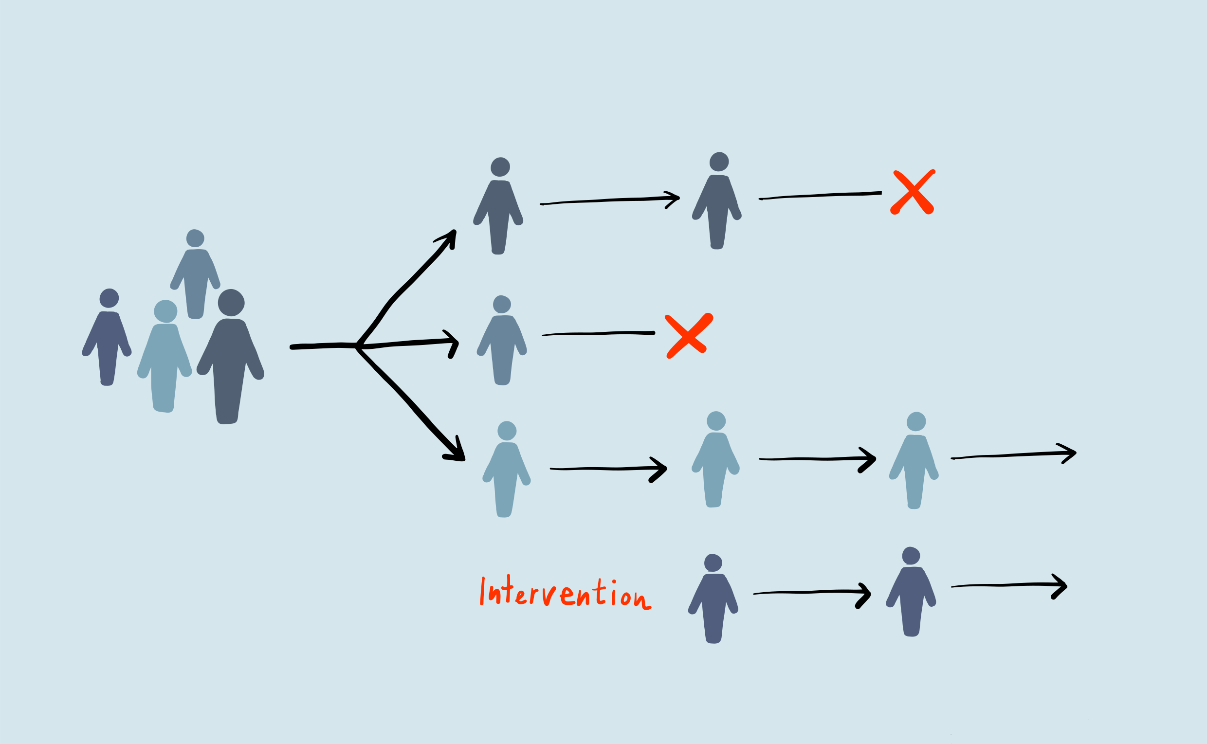
Statistics is the backbone of impactful, reproducible research. Properly done, statistics provide us with basis for cause and effect (known as causal inference). I wanted to write a few supplementary articles for myself and others to understand the basics of probability, statistics, and linear algebra to boost their research. If you get stuck on the notation, please check the Math Notation Sheet. First, an inspiring image from our friends in biostatistics, a sub-field of statistics devoted to creating and applying statistical methods to biological data.
Boxplots and Tukey’s fence
A boxplot, also known as a box-and-whisker plot, is a way to represent numerical data with a visual estimation of the data’s locality (center of the data), spread (from the median), and skewness (asymmetry of the data). It is composed of a box spread across the interquartile range (Q3-Q1), a vertical line at the median (\(\tilde{x}\)), and whiskers capped by fences located at the minimum and maximum of the dataset.
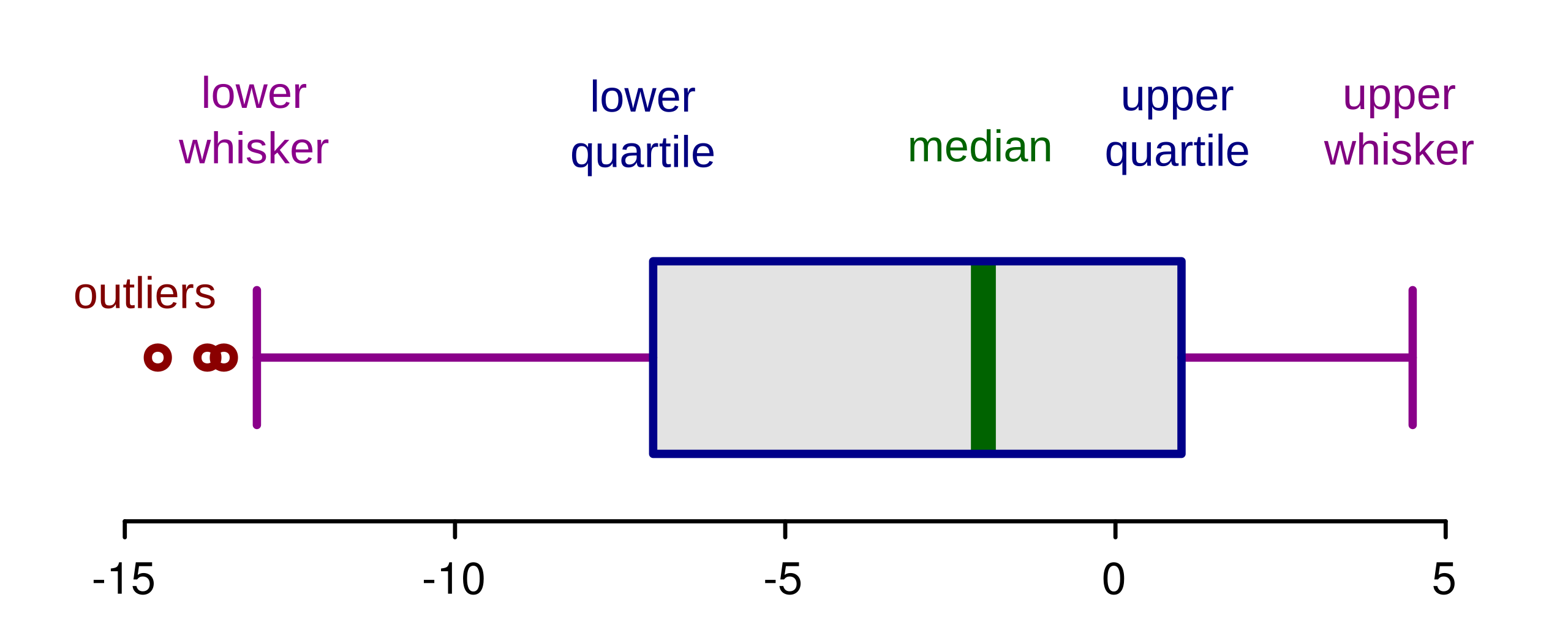
A common heuristic for an outlier are Tukey’s fences, which is defined as \([Q1-k\times IQR, Q3+k\times IQR]\) where \(IQR = Q3-Q1\) and \(k = 1.5\). Another variation of the boxplot is a notched boxplot, which is especially useful when comparing distributions between categories. The notch’s position is often set by \(\tilde{x}\pm \frac{1.58\times IQR}{\sqrt{n}}\).
The design of the boxplot lends itself to easy calculation of summary statistics. The five used by Tukey are discussed below. While the boxplot offers a visual representation of locality, skewness, and spread, here is the mathematical basis of each.
- Locality: mean, median, or mode.
- Skewness: \(\tilde{\mu_3} = \frac{\sum_{i}^{N}(X_i - \bar{X})^3}{(N-1)\times\sigma^3}\) where
\(N\) = number of variables in the distribution
\(X_i\) = random variable
\(\bar{X}\) = mean of the distribution
\(\sigma\) = standard deviation
- Spread: range (max - min), IQR, standard deviation, or variance.
Summary Statistics
The Tukey Five-Number Summary (after the mathematician John Tukey) of a data set consists of the:
- Minimum (Min)
- Quartile I (Q1): 25% of the data are less than or equal to this value
- Quartile 2 (Q2) aka the median: 50% of the data are less than or equal to this value
- Quartile 3 (Q3): 75% of the data are less than or equal to this value
- Maximum (Max)
Standard deviation \(\sigma\), also abbreviated as SD, is a measure of the amount of variation of the values of a variable about its mean. \(\sigma = \sqrt{\frac{1}{N}\sum_{i=1}^{N}(x_i - \bar{x})^2}\) if values \(i\) through \(N\) represent the entire population. If values are selected at random, a correction is applied (Bessel’s correction), such that \(\sigma = \sqrt{\frac{1}{N - 1}\sum_{i=1}^{N}(x_i - \bar{x})^2}\).
Variance is quantifies the spread of data around a sample mean and is just \(\sigma^2\). A higher variance means greater spread.
Sampling Methods
In a simple random sample, every member of the population has an equal chance of being selected is \(\frac{1}{N}\).
In a stratified sample, the population is divided into homogeneous subgroups (strata), and a random sample is drawn from each stratum. This ensures representation across key subgroups.
In a systematic sample, individuals are selected at regular intervals from an ordered list — for example, every \(k^\text{th}\) person, where \(k = \frac{N}{n}\).
Normal Distribution
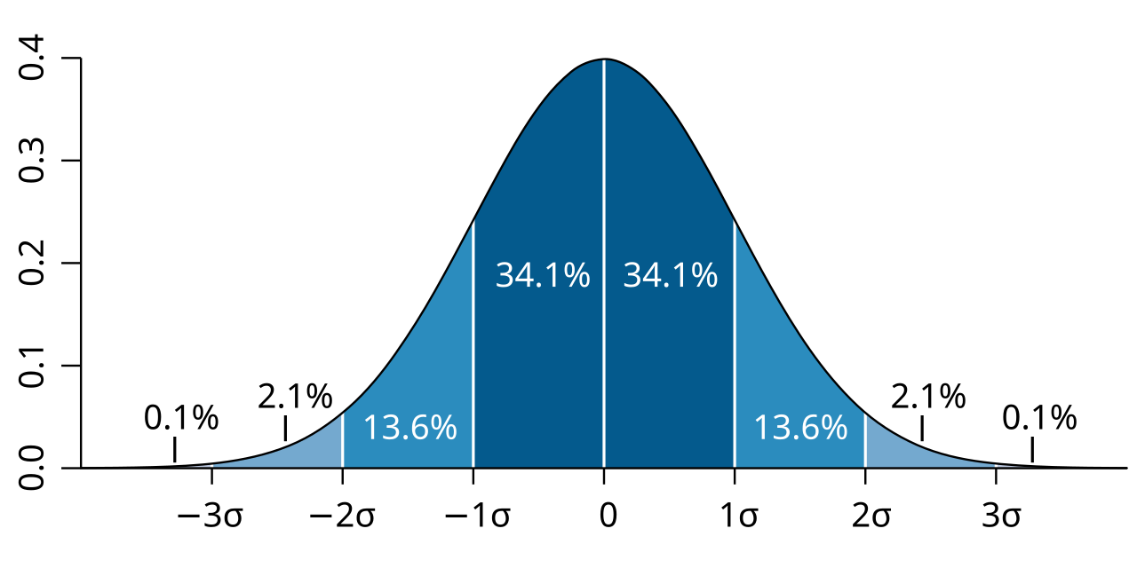
Let’s start with a normal (Gaussian) distribution, also known as a bell curve.
A normal distribution in a variate \(X\) with mean \(\mu\) and variance \(\sigma^2\) is a statistic with probability density function
\(P(x) = \frac{1}{\sigma\sqrt{2\pi}}e^{\frac{-(x-\mu)^2}{2\sigma^2}}\) on the domain \(x\in(-\infty, \infty)\).
To illustrate, assume the mean \(\mu = 0\) and the variance \(\sigma^2 = 1\). \(\sigma\) alone is the standard deviation (the square root of the variance). Therefore, when \(x = 0\), \(P(x)\) is \(\frac{1}{1\sqrt{2\pi}}e^{\frac{-(0-0)^2}{2(1)^2}} = \frac{1}{1\sqrt{2\pi}}\).
A Z-score is quantified as the number of standard deviations a value falls away from the sample mean. To calculate a Z-score \(z = \frac{x - \mu}{\sigma}\) where \(\mu\) is the mean of the population, and \(\sigma\) is the standard deviation of the population.
The Z-score can help us describe the normal distribution in quantiles. The empirical rule (68-95-99.7 rule) of the normal distribution states that approximately 68% of the data falls within 1 SD of the mean, 95% within 2 SD, and 99.7% within 3 SD of the mean.
Looking Ahead
I hope these formulas help you understand how summary statistics are calculated, such as the skewness, standard deviation, or variance.
Stay tuned for next time, where we will cover the basics of probability. Future posts will cover hypothesis testing, linear models, and dimensionality reduction. Stay curious!